Inflation – Unemployment Trade-off — Introduction

Inflation – Unemployment Trade-off — Introduction

Inflation and Unemployment – Keynesian Model of Economy –

In simple Keynesian model of economy, the aggregate supply curve (with variable price level) is of inverse L – shape, it is the horizontal straight line up to the full employment level of output. During the recession or depression the economy has excess capacity and large scale unemployment of labour and idle capital stock, the aggregate supply curve is perfectly elastic. When full employment level of output is reached, aggregate supply curve becomes perfectly inelastic.

In simple Keynesian model, increase in aggregate demand before the level of full employment, causes increase in the level of real national output and employment with price level remaining unchanged.

In the Keynesian model, once the full employment level of output is reached and aggregate supply curve becomes vertical, further increase in aggregate demand caused by the expansionary fiscal and monetary policies will only raise the price level in the economy. In simple Keynesian model inflation occurs in the economy only after full employment level of output has been attained.

So, in the simple Keynesian model with inverse L – shaped aggregate supply curve there is no trade-off between inflation and employment.

Inflation – Unemployment Trade-Off — Phillips Curve –

A British economist, A.W. Phillips published an article in 1958 based on his research using historical data from the U.K. for about 100 years in which he arrived at the conclusion that there is an inverse relationship between rate of unemployment and rate of inflation. This inverse relation implies a trade-off, that is, for reducing unemployment, price in the form of a higher rate of inflation has to be paid, and for reducing the rate of inflation, the price in terms of a higher rate of unemployment has to be borne.

On graphically fitting a curve to the historical data Phillips obtained a downward sloping curve showing the inverse relation between rate of inflation and rate of unemployment and this curve is named after his name as Phillips Curve.

This Phillips Curve shows, rate of unemployment on horizontal axis and rate of inflation on vertical axis.

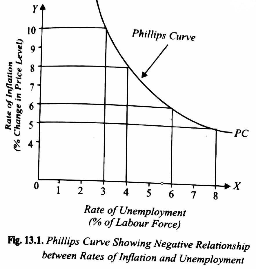
It is seen (in above fig. 13.1) that when rate of inflation is 10 percent, the unemployment rate is 3 percent, and when the rate of inflation is reduced to 5 percent per annum (say by pursuing contractionary fiscal policy and thereby reducing aggregate demand), the rate of unemployment increases to 8 percent of the labour force.

The actual Phillips Curve drawn from the data of sixties (1961-69) for the United States also shows the inverse relation between unemployment rate and inflation rate.

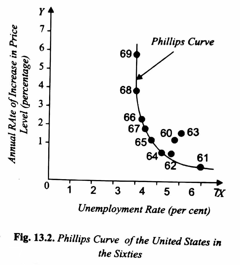
On the basis of this, many economists came to believe that there existed a stable Phillips Curve which depicted a predictable inverse relation between inflation and unemployment. Further, on the basis of a stable Phillips Curve for a country, they emphasized the trade-off that confronts the economic policy makers. This trade-off presents a dilemma for the policy makers, should they choose a higher rate of inflation with lower unemployment or a higher rate of unemployment with a low inflation rate.

During seventies a strange phenomenon was witnessed by the USA and Britain when there existed a high rate of inflation side by side with high unemployment rate. This was contrary to both Phillips curve concept and the simple Keynesian model. This simultaneous existence of both high rate of inflation and high rate of unemployment has been described as Stagflation.